Modeling Load Within a Dynamic Voltage Scaling Application
Overview
This example shows how, depending on the workload, a AT90S8535 microcontroller uses a dynamic voltage scaling (DVS) feature to adjust the input voltage. By lowering the input voltage when the workload is low, the microcontroller reduces energy consumption while guaranteeing quality of service. The DVS controller is based on an online gradient estimation technique called infinitesimal perturbation analysis (IPA). In a single simulation of a parameterized system, not the large number of simulations required by a traditional finite-difference approach, IPA can provide sensitivity information that yields a first-order approximation of the system performance metrics as a function of the parameters.
Applying IPA to the Controller
The performance metric to minimize is the average cost per job, given by
![$$J(\theta)=wP(\theta)+S(\theta)=wc_{2}\left[V_{t}/\left(1-c_{1}/\theta \right) \right]^{2}+S(\theta)$$](../../examples/simevents/win64/DynamicVoltageScalingExample_eq06728943162783552755.png)
where
 is the average service time of a job, which is a function of the input voltage V. That is, finding the optimal value of also yields the optimal value of V.
 is a weighting constant.
 is the average energy consumption of a job in Joules.
 is the average system time for jobs, which measures quality of service. This model uses an M/M/1 queuing system, so a closed-form expression for provides a way to compare the IPA results in the simulation with theoretical results.
 and
and  are device-dependent constants.
 is the device minimum input voltage.
To find a value of for which  is 0, this model uses a gradient method with constant step size
  . The
. The  th iteration of the optimization, which occurs upon the departure of the th job, uses the estimate
  to produce
To learn about the IPA estimation of  , see the works listed in References.
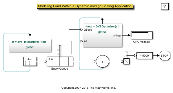
Structure of the Model
The model includes these components:
Job Arrivals section: Provides source of jobs that form the workload
FIFO Queue, Single Server, and other blocks in the blue section: Provides queuing for jobs in the system
DVS Optimizer subsystem: Uses the queue length,
value, service time for the latest job, and total number of jobs to compute  and the corresponding updated input voltage.
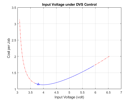
Results and Displays
The model includes these visual ways to understand its performance:
A dynamic plot showing how the DVS controller varies the voltage during the simulation to reduce the average cost per job.
A Display block that shows the average service time for jobs.
A Display block that shows the corresponding input voltage.
To experiment, try changing the value of the Avg Interarrival Time block before running the simulation.
References
[1] Cassandras, C. G., and S. Lafortune. Introduction to Discrete Event Systems. Boston, MA: Kluwer Academic Publishers, 1999.
[2] Li, W., C. G. Cassandras, and M. I. Clune. "Model-Based Design of a Dynamic Voltage Scaling Controller Based on Online Gradient Estimation Using SimEvents." Proceedings of 45th IEEE Conference on Decision and Control. 2006, pp. 6088-6092.
[3] Weiser, M., B. Welch, A. Demers, and S. Shenker. "Scheduling for Reduced CPU Energy." Proceedings of the 1st Symposium on Operating Systems Design and Implementation. 1994, pp. 13-23.
See Also
Entity Generator | Entity Server | Queue | Resource Pool | Resource Acquirer | Resource Releaser
Related Topics
You can also select a web site from the following list:
Americas
- América Latina (Español)
- Canada (English)
- United States (English)
Europe
- Belgium (English)
- Denmark (English)
- Deutschland (Deutsch)
- España (Español)
- Finland (English)
- France (Français)
- Ireland (English)
- Italia (Italiano)
- Luxembourg (English)
- Netherlands (English)
- Norway (English)
- Österreich (Deutsch)
- Portugal (English)
- Sweden (English)
- Switzerland
- United Kingdom (English)